XMATCH Function Excel

XMATCH Function

The XMATCH function in Excel returns the position of an item in an array. By default, an exact match is required. The syntax for the XMATCH Function is:

=XMATCH(lookup_value, lookup_array, [match_mode], [search_mode])

Breakdown of the inputs (arguments). The inputs with parenthesis [ ] are optional:

• Lookup_value: the value you’re interested in finding within the dataset
• Lookup_array: the dataset where you can find the lookup value. This is typically a column.
• [match_mode]: choose the type of match. Options are: exact, exact or next smaller, exact or next larger, and wildcard match (we’ll cover these in examples below).
• [search_mode]: choose the search mode. Option are: first to last, last to first, or sorted ascending or descending.

Now that we understand the syntax, let’s look at some examples from easy to hard. 

XMATCH Example 1 (Basic)

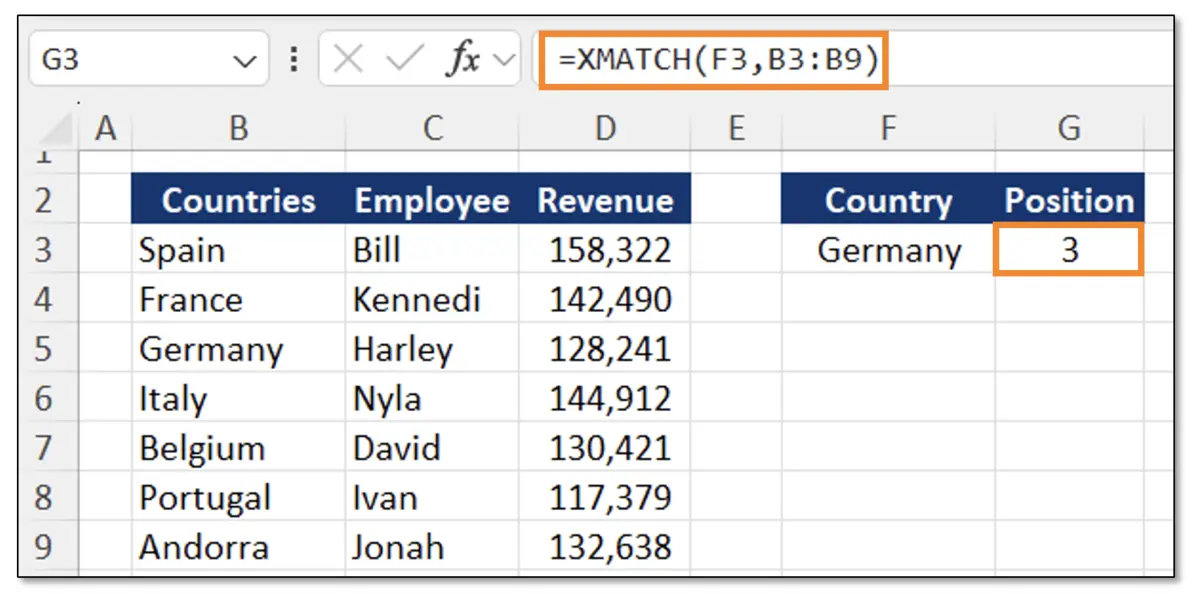
In the table above, suppose you want to find the location of Germany within the list of countries. For this, we would select Germany in cell F3 as the lookup_value, and the range B3:B9 as the lookup_array. This will give us an answer of 3, as Germany is located in third position within the list of countries.

The XMATCH function used in this scenario is not very useful. So let’s explore more relevant examples below.

XMATCH Example 2 (Intermediate)

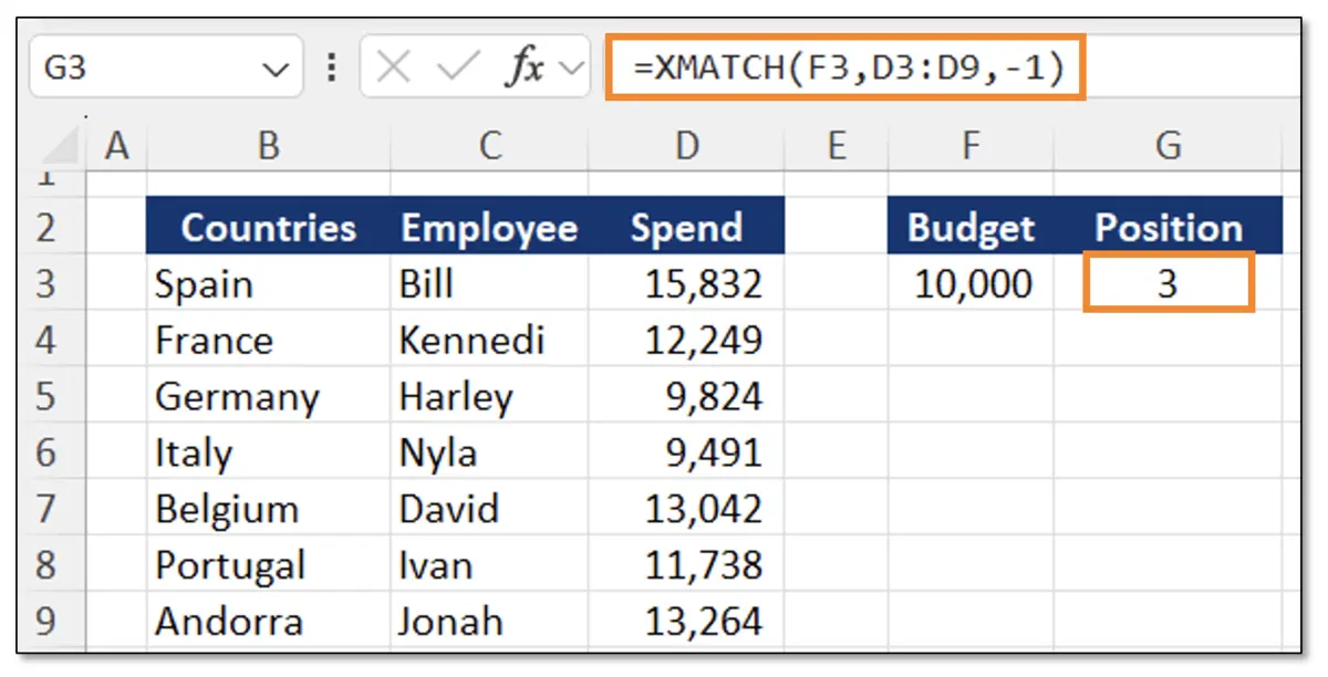
In the table above, suppose we want to know who got closest to our budget of $10,000 without surpassing it. For this, we can use the XMATCH Function with the match_mode. As the match_mode option, we’ll use the -1 which stands for the exact match or next smaller item. 

This helps us find who came closest to reaching full budget without surpassing it. In this case, it’s Harley from Germany. 

XMATCH Example 3 (Advanced)

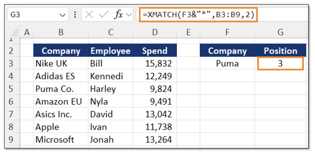
What happens if we don’t know the exact name? For example, companies often have names such as Nike Inc. for Nike, or Puma Co. for Puma. Is there a way for us to use the XMATCH in this scenario? Yes! That’s where the wildcard match_mode comes handy. 

For this, suppose we want to find the position of Puma within the table. However, you’ll notice that Puma is not an exact match, as it’s written as Puma Co. in the data table. To work around this, we’ll use the XMATCH with a Wildcard. 

First, add the lookup_value, and at the end of the cell, add an ampersand (&) and an asterisk (*) between quotations (“ “). This tells Excel that anything after the lookup_value can be ignored. Now, we just need to add the number 2 under the search mode to activate the wildcard. 

The result is position 3, despite Puma and Puma Co. not being exact matches. 

XMATCH Example 4 (Expert)

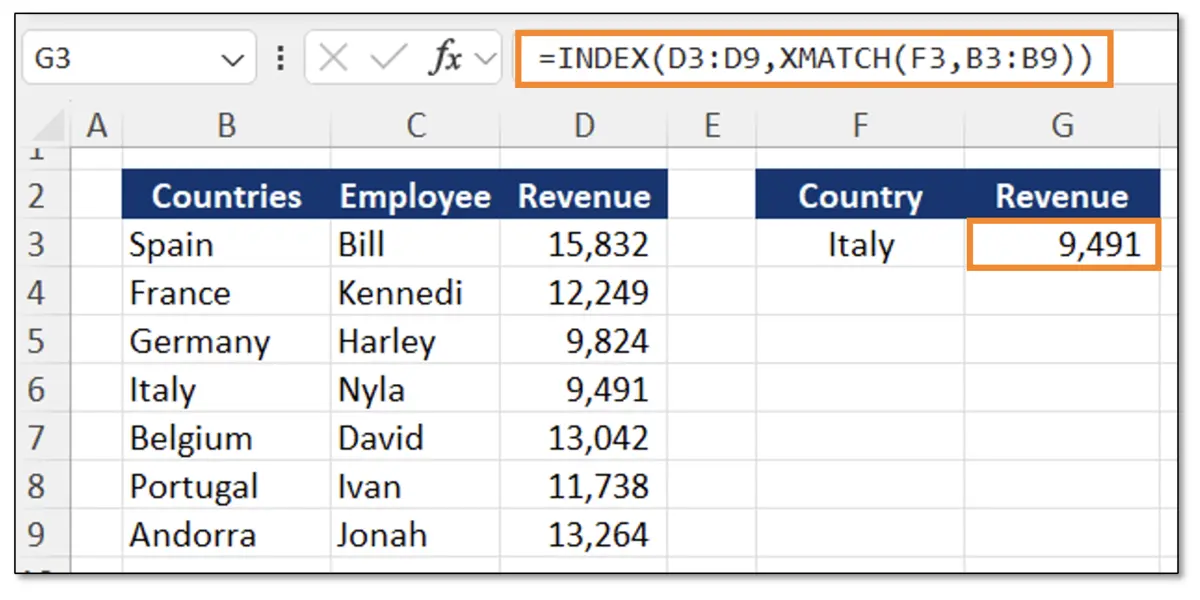
The XMATCH function is most useful when combined with other Excel functions such as the INDEX. So let’s look at an example below:

In the table above, we want to find the revenue for Italy. If we only used the XMATCH function, it would give us the position, and not the actual amount of revenue. That’s where the INDEX XMATCH combination comes handy.

In the INDEX function, we first add the array which is the result array (in this case the revenue figures). Then, as the row_num we add the XMATCH function. Adding a function inside of another function is known as nesting in Excel. The syntax for the XMATCH is the same as the previous examples. 

The final result is the revenue amount, instead of the position number we would have gotten just by using the XMATCH function.  

XMATCH Function Errors

The XMATCH Function can show an #N/A error when there is no match. For example, if you’re looking for “Sam” within a column of names, and “Sam” is not a name in that column, it will give the #N/A error.

The #VALUE! error happens when there’s an error in the values added to the formula. For example, in the match_mode, if you added a 3, which is not an option that’s available, it would return a #VALUE! error. 

XMATCH vs MATCH Functions

The XMATCH is the successor of the MATCH function in Excel. The XMATCH is more flexible with features such as the search mode allowing you to search in different orders, and the wildcard match mode for partial matches of a value.

Alternatives to the XMATCH

Instead of finding the position number, if you’re interested in finding the actual value in that position, the XLOOKUP function is probably the easiest solution. 

Another option that’s arguably more difficult is the INDEX MATCH function as it requires two separate formulas (the INDEX and the MATCH) to make it work.

Additional Resources

If you found this article useful, consider checking out our Excel for Business & Finance Course, where we help students learn the technical skills needed to perform in competitive finance and investment roles. Use this course to join our students who have landed roles at Goldman Sachs, Amazon, Bloomberg, and other great companies! 

Other Articles You Might Find Helpful

• XLOOKUP Function
• INDEX MATCH Function
• SUMIFS Function
• COUNTIFS Function
• IFERROR Function