

COUNTIFS Function in Excel
The COUNTIFS function in Excel counts the number of cells in a range if one or more conditions are true.
Excel COUNTIFS Function (syntax)
The COUNTIFS function in Excel counts the number of cells in a range if one or more conditions are true.
=COUNTIFS(criteria_range1, criteria1,...)
Breakdown of the inputs (arguments):
- Criteria_range1: the range that is being tested by criteria1.
- Criteria1: the criteria that defines which values should be counted from the criteria_range1.
- …: the three dots at the end of the function represent any additional criteria you might have. To add more criteria, simply put a comma key to activate the next criteria range. The minimum number of criteria is one, while the maximum is 127.
If you have multiple criteria, all the conditions must be met (not just one) to be included in the final count. Each new criteria will require choosing a criteria range and a criteria again.
Basic COUNTIFS Example
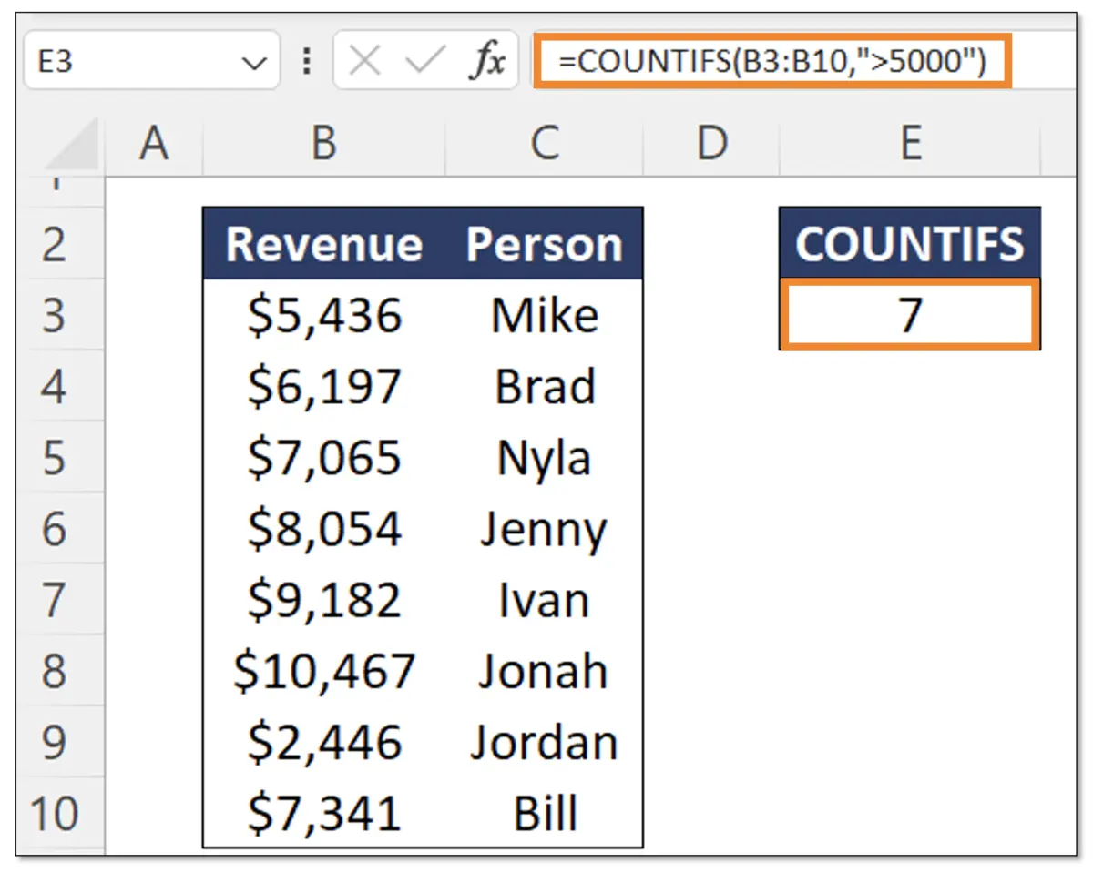
In the table above, suppose we want to find out the count of people with revenue greater than $5000. For this, we can use COUNTIFS with one criteria:
=COUNTIFS(B3:B10”>5000”)
- Criteria_range1: the criteria range we’re interested in. The revenue in this case.
- Criteria1: “>5000” (greater than 5) is the criteria that defines how to filter the criteria_range1 so we only count the revenue instances that are greater than $5000.
The criteria must be wrapped in quotes (“”). In this instance, we used the greater than operator “>” but we can also use the equals, smaller than, or even a combination like greater than or equals to “>=” as well.
COUNTIFS with Multiple Criteria
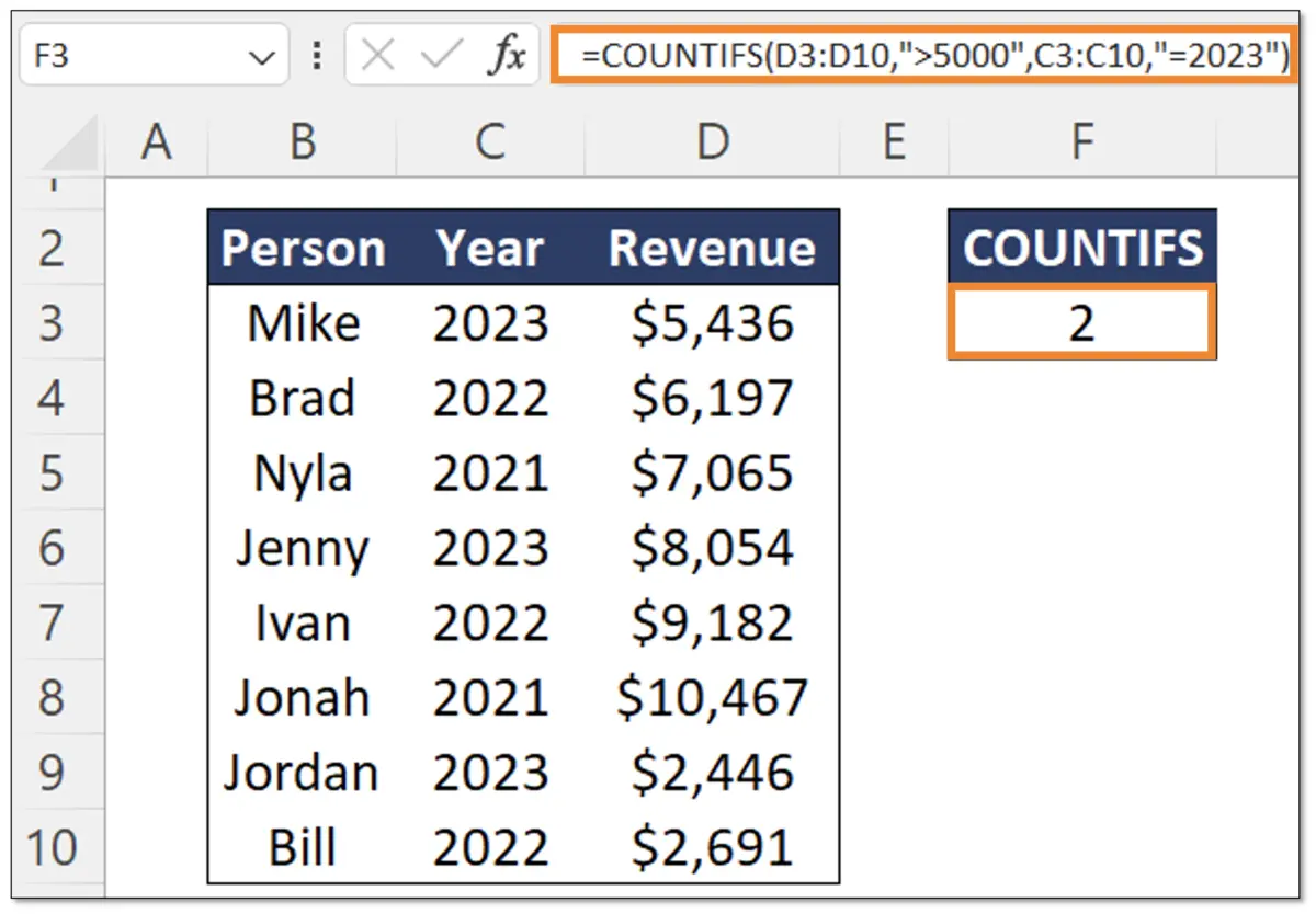
In the table above, we want to find out the count of persons that have revenue greater than $5,000 AND are in 2023. Therefore, we have two criteria this time.
The first criteria and criteria range remains the same as the previous example. However, we now have a second criteria and criteria range. For this, we select the criteria_range2 which is C3:C10. We then set the criteria2 to equal 2023.
While we had two criteria in this example, you use the same pattern for adding multiple criteria. One important note is that the criteria range lengths must always be the same. In this case, both criteria ranges are 8 rows long. If one way 8 rows and the other was 10, the COUNTIFS would not work.
COUNTIFS with Wildcard
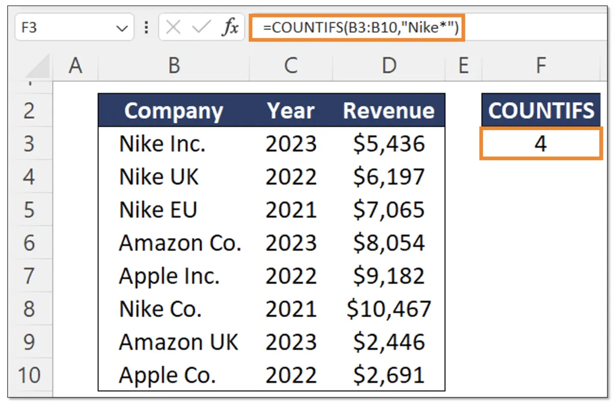
Sometimes data is not easy to work with. For example, in the table above, we have Nike in several different variations such as Nike Inc., Nike UK, Nike EU, etc. What if we just want to find out the count of Nike instances regardless of which version of Nike this is? For this we can use a variation of a COUNTIFS by using the Wildcard feature.
=COUNTIFS(B3:B10”Nike*”)
- Criteria_range1: B3:B10, which is all of the company names.
- Criteria1: “Nike*” Nike is the company name we’re looking for, and the asterisk (*) allows for a match to be similar, instead of exact. So it counts anything that starts with the word Nike first. Therefore, Nike UK, Nike EU, etc. are all included in the count criteria.
COUNTIFS Not Working / Limitations
There are two main limitations to the COUNTIFS Function on Excel.
- Range Size: The range sizes for each criteria range must always be the same. For example, having criteria_range1 with 5 rows and criteria_range2 with 10 will return a #VALUE! error.
- All criteria must be met: To be included in the result, all criteria must be met. The value cannot just meet 1 of the 2 in the COUNTIFS. Instead, all criteria must be met to be included in the result. That said, there is a workaround to have the COUNTIFS count if one condition is met, OR if another condition is met. See the next paragraph for more.
Advanced COUNTIFS (COUNTIFS + OR)
Suppose we want the COUNTIFS to show the result if at least one condition is true. Even if there is more than one condition, if at least one is met, we want to include it in the result. For this we can add two or more COUNTIFS.
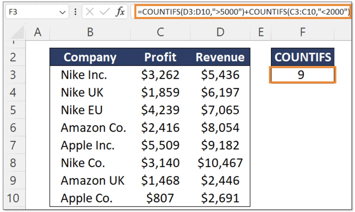
In the table above, we want to find the count if the revenue is greater than $5,000 or if the profit is less than $2,000. This can be done by adding two COUNTIFS together.
=COUNTIFS(D3:D10,">5000")+COUNTIFS(C3:C10,"<2000")
By adding the two COUNTIFS, we tell Excel to show the result if at least one of the two conditions is true. In this case, the conditions are that the revenue be greater than $5,000 OR that the profit be smaller than $2,000.
Similar Functions to COUNTIFS
Some useful alternatives to the COUNTIFS function are the SUMIFS, AVERAGEIFS, and SUMPRODUCT.
- SUMIFS: Sums a range if one or multiple conditions are true.
- AVERAGEIFS: Calculates the average of a range if one or multiple conditions are true.
- SUMPRODUCT: Multiplies ranges and returns the sum of products. This is often used to calculate the weighted average.
Additional Resources
If you’re interested in learning more Excel, consider checking out our Excel for Business & Finance Course where we help students learn to use Pivot Tables, Lookup formulas, data cleaning tools, and other helpful Excel functions. Use this course to join our students who have landed roles at Goldman Sachs, Amazon, Bloomberg, and other great companies!
Other Articles You Might Find Helpful


Ready to Level Up Your Career?
Learn the practical skills used at Fortune 500 companies across the globe.