Excel Sort Function

Usage:

Use this formula to sort a range of data (also known as a list or array of data).

The SORT formula is perfect for users looking to reorganize their data sets in a logical, easy-to-follow manner. Some common sort types include alphabetical sort (A-Z) or chronological sort (oldest to newest).

Function Layout (Syntax):

=SORT(array, [sort_index], [sort_order], [by_col])

Inputs (Arguments):

• Array: The base set of cells to sort.
• [Sort_index]: Column index number. The sort function allows users to indicate which column to sort by (the first column from the left is 1, the second column from the left is 2, etc.). Default option is to sort by the first column from the left.
• [Sort_order]: Ascending or descending order. Ascending order (A-Z or Oldest to Newest) is represented by a 1 and descending order (Z-A or Newest to Oldest) is represented by a -1. Default option is to sort by ascending order.
• [By_col]: Sort by column instead of row. If you input “TRUE” you can switch the function to sort by column while the input “FALSE” sorts the range by rows. The default option is to sort by rows.

Example: Simple Sort

Let’s start with a basic example where we’ll sort a table with customer purchase data.

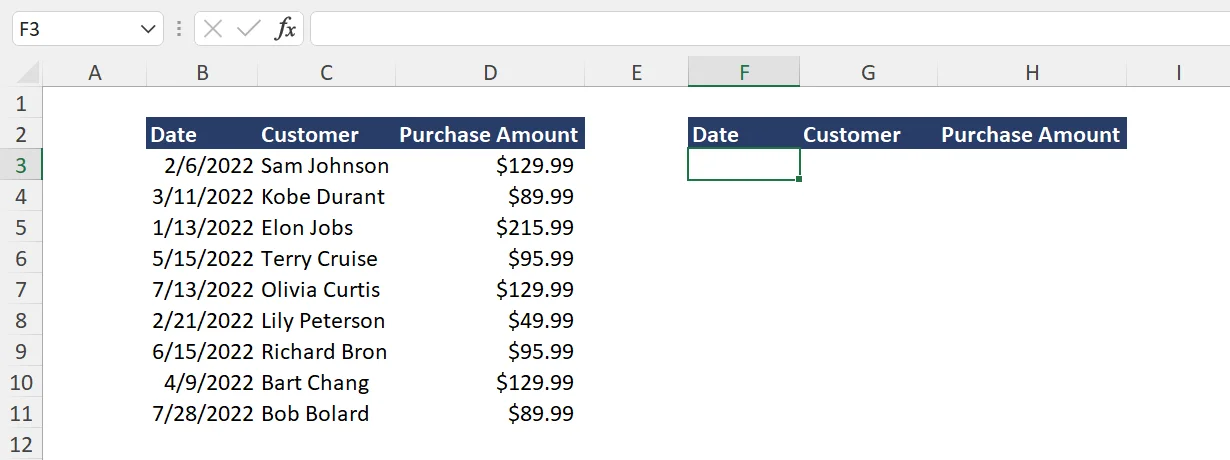
In this particular example, we have a table containing the purchase date, customer name, and purchase amount. Let’s sort the table by purchase date from oldest to newest by following these steps:

1. Initiate the formula by typing “=SORT(“.
2. Fill in the array input. This should be cells B3:D11.
3. Ignore the other optional inputs and close the function. You should see a table sorted from oldest purchase dates to newest purchase dates.

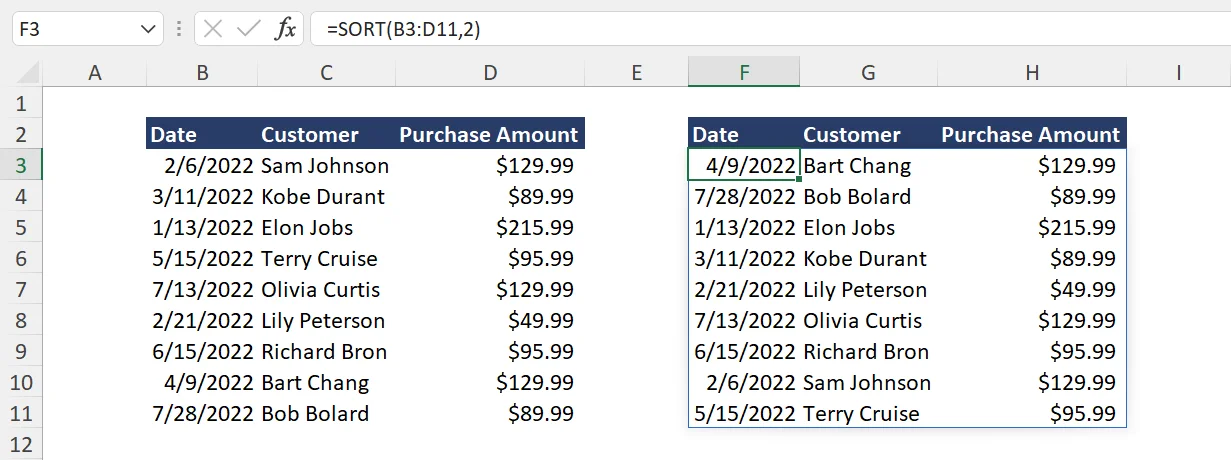
=SORT(B3:D11)

Notice how we only input the array argument and ignore all of the other optional inputs. This tells the function to use the default settings for the other optional inputs (sort by first column, sort by ascending order, and sort by rows).

Example: Sorting Second Column

Now let’s try another example where this time we’ll use the optional input [sort_index]. This optional input allows you to tell Excel which column you want to sort by. If you want to sort by the first column from the left type 1, for the second column type 2, third column type 3 … and so on and so forth.

In this particular example, we’ll sort the table by the second column instead of the first column. To do this, simply set [sort_index] = 2.

=SORT(B3:D11,2)

Example: Ascending vs Descending Order

Now let’s continue the previous example by adding on another optional input, [sort_order]. Sort order allows you to tell Excel to sort by ascending or descending order.

In this particular example, we’ll change the default sort and use descending order by typing in -1.

=SORT(B3:D11,2,-1)

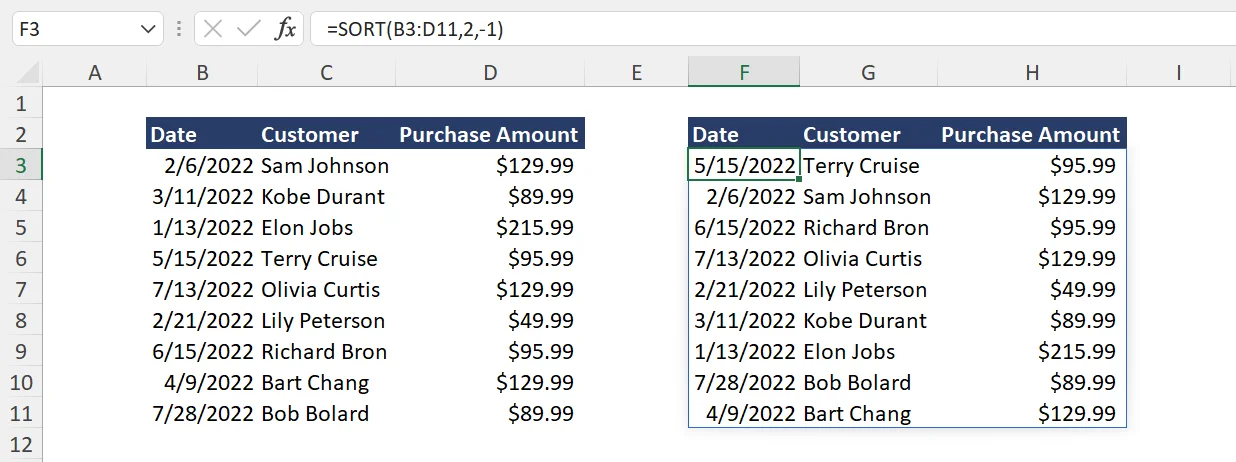
By using this sort function, we have essentially told Excel to sort the customer names (second column) by descending order (Z-A).

Example: Sorting by Column

Now let’s take a look at a different example where we’ll sort by column.

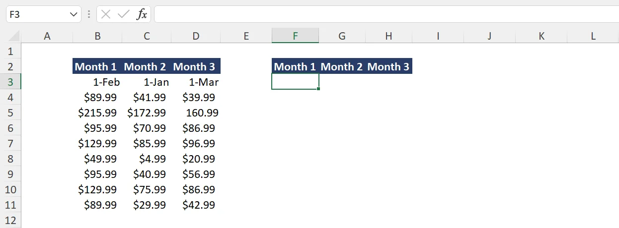
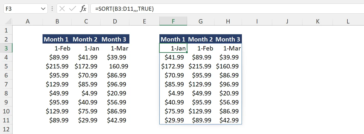
In this case, we have 3 columns of sales data. Here, we’ll use the sort function to sort the columns chronologically so that we have January first, followed by February, then March.

To do this, we’ll skip the other optional inputs and simply enter “TRUE” for the [by_col] input.

=SORT(B3:D11,,,TRUE)

Example: Sort + Filter Function

The SORT function is commonly combined with the FILTER function when users want to filter a dataset and sort the dataset in one step.

Let’s take a look at how this works by revisiting our first example. Let’s say in this particular instance, we’ll want to sort for purchases greater than $90 then sort those purchases from greatest to smallest.

Step 1 

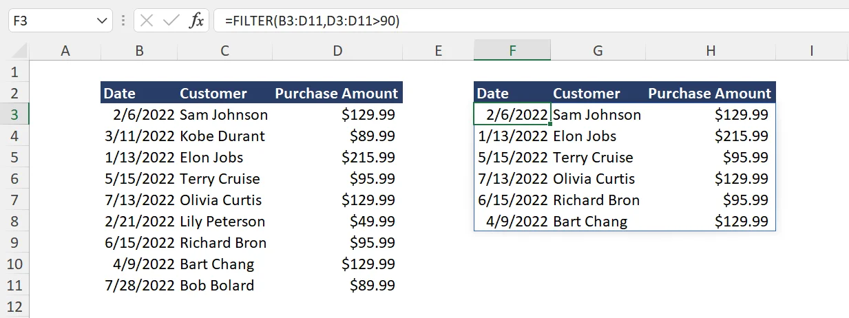
Step 1 is to first implement the filter function. This can be done by selecting the initial data range and setting the filter criteria where the purchase amount (column D) is greater than $90.

=FILTER(B3:D11,D3:D11>90)

Step 2

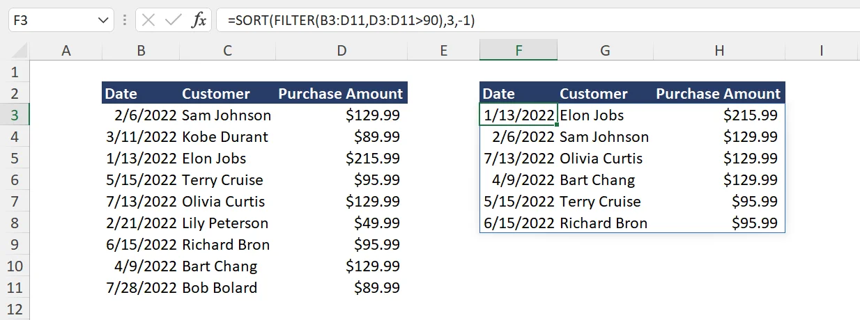
Now that you have the filtered list in place, you can wrap the SORT function around the FILTER function to start your sort. In this case, we want to sort by purchase amount (3rd column) in descending order (represented by -1).

=SORT(FILTER(B3:D11,D3:D11>90),3,-1)

Additional Resources:

If you’re interested in further developing your Excel skills to better your chances of landing a competitive business or finance role, check out our Excel for Business & Finance Course and more using the get started button below.

Other Articles You May Find Helpful:

• Excel Filter
• How to Prepare an Income Statement
• Interview with a Tesla Financial Analyst
• Must Know Finance Interview Questions